Estimating HPL Performance: from Theoretical Peak to Deliverable Efficiency

Abstract: After computing Rpeak, everyone asks "what will it actually deliver?" This article answers with real per-node HPL data from a 91-node cluster: single-node efficiency, scaling loss at 36/80 nodes, and a practical estimation formula.

1. The Metric: Efficiency

$$\eta = \frac{\text{Measured GFlops}}{\text{Theoretical Rpeak}}$$

• Single-node efficiency: tuning quality (BIOS, binding, ISA)
• Cluster efficiency: adds interconnect, load balance, and HPL grid effects

2. Real Baseline: 91-Node Per-Node Results

Uniform nodes: 104 cores @ 2.0 GHz, 6656 GFlops/node, 1536 GB/node.

2.1 Result distribution

Stat	Value
Theoretical peak	6656 GFlops
Best measured	6433.05 GFlops (96.6%)
Worst measured	5777.46 GFlops (86.8%)
Average measured	~6218 GFlops
Average efficiency	93.4%

Nodes below ~90% should be investigated individually (memory quality, thermals, aging); acceptance uses the cluster average but flags outliers.

2.2 Efficiency bands

Band	Measured (GFlops)	Typical case
96%+	6389+	well-tuned, good silicon
93%~95%	6189~6323	majority of nodes (average)
90%~93%	5990~6189	acceptable, watch
<90%	<5990	check memory / cooling / throttling

3. Memory Bandwidth Efficiency (Often Overlooked)

Same nodes, STREAM-style test:

$$\text{Theoretical BW} = 563200 \text{ MB/s}$$

Measured ~418000 MB/s → 74.2% — typical for DDR platforms (70–80% is normal).

Metric	Theoretical	Measured	Efficiency
Memory BW	563200 MB/s	~418000 MB/s	74.2%

4. Scaling Efficiency: 36 and 80 Nodes

Scale	Rpeak	Measured	Efficiency	Runtime
1 node (avg of 91)	6656	~6218	93.4%	tens of minutes
36 nodes	239616	191494	79.9%	~58 min
80 nodes	532480	417170	78.3%	~13.8 h

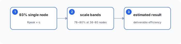
Key fact: the 93% single-node baseline drops to 78–80% at 36–80 nodes. Communication and load imbalance cost efficiency at scale — never extrapolate single-node efficiency to a full cluster.

5. Estimation Formula

For $N_{\text{node}}$ nodes with per-node peak $Rpeak_{\text{node}}$:

$$\text{Estimate} = Rpeak_{\text{node}} \times N_{\text{node}} \times \eta_{\text{scale}}$$

Empirical $\eta_{\text{scale}}$ by size:

Scale	Suggested η	Notes
1 node	90%~93%	93% when well tuned
8~16 nodes	85%~88%	comm overhead appears
32~64 nodes	80%~84%	typical
80~128 nodes	78%~82%	large-scale ceiling
256+ nodes	75%~80%	needs careful P×Q tuning

6. Tool: N_calculator Efficiency Table

*** 70% --> 4659.20     *** 80% --> 5324.80     *** 90% --> 5990.40  ***
*** 93% --> 6189.44     *** 95% --> 6323.20     *** 100%--> 6656.0   ***

7. Practical Flow

1. Estimate first: use 93% (single node) and 78% (80 nodes) in your delivery plan.
2. Verify by testing: single-node tuning → small scale (2/4/8) to see the curve → full scale once.
3. Report all three numbers: theoretical, measured, efficiency — unambiguous.

8. Takeaway

• ~93% single-node HPL efficiency is the realistic x86 (AVX-512 + MKL) expectation.
• ~78–80% at 80 nodes; estimate per scale band, not flat.
• Memory bandwidth (~74%) is recorded separately from HPL efficiency.

Next: the real measurement run — CPU HPL in Practice: from Single Node to 80 Nodes.